A quick start on using plag package
plag is written in python/cpython. The base calculations are done in cpython (_plag.pyx) to make it fast. A python wrapper (plag.py) is used to manage the calls.
The files are not well documented yet. This tutorial walks through a simple example of calculating the psd and lags between two light curves in the file named data.lc in the current directory.
- We import numpy and our plag packages.
- We call pylab to help with plotting.
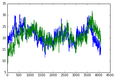
- We then read the light curve data. The file has 5 columns: time, lc1, lc1e , lc2, lc2e. These are simulated light curves with a high signal and no gaps to illustrate the general use of the package.
- The light curves are then plotted.
import numpy as np
import plag

## for plotting ##
%pylab inline

### read the light curve ###
data = np.loadtxt('data.lc')
dt = data[1,0] - data[0, 0]

_ = plot(data[:,0], data[:,1])
_ = plot(data[:,0], data[:,3])
Populating the interactive namespace from numpy and matplotlib

Prepare the data
Because the light curves are long, we split them to segments of length seg_length=256, and then create a list of segments to be passed to the clag initializer.
# Split the light curve into segments #
seg_length = 256
index = np.arange(len(data)).reshape((-1, seg_length))

T = [data[i, 0] for i in index]
Lc1  = [data[i, 1] for i in index]
Lc1e = [data[i, 2] for i in index]
Lc2  = [data[i, 3] for i in index]
Lc2e = [data[i, 4] for i in index]
- We now define the frequency bins to be used for the psd and cross spectrum calculations.
#### Get the psd for the first light curve ####

# frequency bins #
fqL = np.logspace(np.log10(1.1/seg_length),np.log10(.5/dt),7)
fqL = np.concatenate(([0.5/seg_length], fqL))
nfq = len(fqL) - 1
Calculate the psd of the first light curve
When modeling a single light curve, we can use plag.psd or plag.lag. When modeling multiple light curves at the same time, use plag.PLag('psd',...) and plag.PLag('lag', ..)
The rest of parameters depend on the class used. To see the parameters do plag.psd? for documentation
plag.PLag is more general so we use it.
To calculate the psd, we need a list of arrays T for the light curve times, Lc1, for the light curve rates, and Lc1e for the light curve measurement errors, then dt, the time bin of the data (i.e. exposure time), and fqL: a list of the frequency boundaries for the bins to be fitted
## initialize the psd class for multiple light curves ##
## the default normalization is rms units ##
P1  = plag.PLag('psd', T, Lc1, Lc1e, dt, fqL)
inpars is a starting array holding the input psd values at the chosen frequency bins, this should have a length len(fqL)-1.
We then print the log likelihood at these input values as a test that things are ok.
## initial parameters, start with ones
inpars = np.ones(nfq)

## print the loglikelihood for the input values ##
print(P1.logLikelihood(inpars))
-20766.7467472
We now do the fitting using plag.optimize, which takes as arguments, the class we just defined, and the input array (plus other arguments to control the fit). This uses a quadratic approximation to the likelihood, and loops until a best fit value is found. The result is returned as a tuple of best fit values, psd1, and their ESTIMATED error psd1e taken from the hessian of the likelihood function. This estimate is generally a lower limit only, and MCMC chains are needed to get the full errors.
The progress is printed with each line showing:
- iteration number.
- maximum absolute change in the parameters in current iteration (absmax).
- maximum absolute gradient at current location (gmax).
- the loglikelihood value.
- a list of fitted parameters
Then once absmax or gmax is below the tolerance level passed to optimize (default 1e-4), or number of iterations exeeds a maximum (default 500), the function prints:
- current parameters
- their estimated errors.
- the gradient at current location The fit is valid if the gradients are close to zero.
## Now do the fitting and find the best fit psd values at the given frequency bins ##
psd1, psd1e = plag.optimize(P1, inpars)
   1 4.466e+02 5.510e+03 inf -- -2.077e+04 -- 1 1 1 1 1 1 1
   2 2.156e-01 3.890e+01 1.594e+04 -- -4.831e+03 -- 447.65 197.72 59.326 23.6258 5.708 1.79856 0.689895
   3 2.356e-02 6.354e-02 1.712e+00 -- -4.829e+03 -- 544.148 192.607 59.8723 21.1887 5.54487 1.73612 0.671665
   4 2.883e-03 2.918e-03 6.352e-03 -- -4.829e+03 -- 556.97 193.207 59.8523 21.1068 5.53967 1.73617 0.671694
   5 3.822e-04 3.719e-04 9.076e-05 -- -4.829e+03 -- 558.576 193.263 59.8235 21.1019 5.53928 1.73617 0.671693
********************
558.576 193.263 59.8235 21.1019 5.53928 1.73617 0.671693
136.107 10 9.32986 2.13858 0.375107 0.0790134 0.0211839
1.14419e-05 6.48102e-06 -7.15781e-05 -7.25802e-05 -0.000234608 -0.000159413 -0.000371948
********************
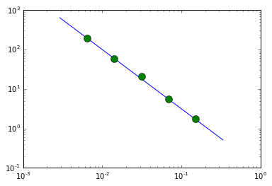
Plot the result of the psd fit
## plot ##
fqd = 10**(np.log10( (fqL[:-1]*fqL[1:]) )/2.)

loglog(fqd, 0.1*fqd**(-1.5), label='input psd')
errorbar(fqd[1:-1], psd1[1:-1], yerr=psd1e[1:-1], fmt='o', ms=10, label='fit')
<Container object of 3 artists>

## Now do the second light curve

P2  = plag.PLag('psd', T, Lc2, Lc2e, dt, fqL)

psd2, psd2e = clag.optimize(P2, inpars)
   1 3.209e+02 4.473e+03 inf -- -1.951e+04 -- 1 1 1 1 1 1 1
   2 2.149e-01 3.308e+01 1.468e+04 -- -4.824e+03 -- 321.904 226.369 58.9332 23.2201 5.73063 1.79719 0.680492
   3 3.297e-02 7.245e-02 1.341e+00 -- -4.823e+03 -- 391.092 214.942 60.6903 20.8544 5.57654 1.76492 0.665351
   4 6.307e-03 1.337e-03 1.049e-02 -- -4.823e+03 -- 403.985 213.446 60.4228 20.8267 5.57309 1.76495 0.665383
   5 1.299e-03 2.276e-04 4.305e-04 -- -4.823e+03 -- 406.533 213.115 60.3338 20.8259 5.57291 1.76496 0.665383
   6 7.001e-05 4.784e-05 1.869e-05 -- -4.823e+03 -- 407.061 213.045 60.3143 20.8259 5.57288 1.76496 0.665383
********************
407.061 213.045 60.3143 20.8259 5.57288 1.76496 0.665383
10 10 9.39487 10 0.377197 0.080288 10
9.91518e-06 -4.04952e-06 -4.78438e-05 -7.71374e-06 -3.72828e-05 4.34726e-05 -3.23287e-06
********************
### Now the cross spectrum ###
### We also give it the calculated psd values as input ###
Cx = plag.PLag('lag',
               [list(i) for i in zip(T,T)],
               [list(i) for i in zip(Lc1,Lc2)],
               [list(i) for i in zip(Lc1e,Lc2e)],
               dt, fqL, psd1, psd2)

inpars = np.concatenate( (0.3*(psd1*psd2)**0.5, psd1*0+1.) )
p, pe = clag.optimize(Cx, inpars)
phi, phie = p[nfq:], pe[nfq:]
lag, lage = phi/(2*np.pi*fqd), phie/(2*np.pi*fqd)
cx, cxe   = p[:nfq], pe[:nfq]
   1 2.328e+00 1.749e+03 inf -- -8.763e+03 -- 143.051 60.8739 18.0205 6.28904 1.66682 0.525152 0.200559 1 1 1 1 1 1 1
   2 1.042e+01 1.672e+03 3.379e+03 -- -5.384e+03 -- 249.98 193.608 59.5574 20.9046 5.54789 1.73941 0.503299 -0.0343698 0.816594 0.923578 1.02812 0.991901 0.967044 0.451682
   3 5.903e-01 8.530e+02 2.730e+02 -- -5.111e+03 -- 228.398 199.138 59.9075 20.9544 5.554 1.73856 0.489617 0.323769 0.989329 0.991401 1.00313 0.998086 0.99099 0.795839
   4 4.193e-01 3.000e+02 8.294e+01 -- -5.028e+03 -- 249.061 202.456 60.0618 20.962 5.55402 1.73902 0.520802 0.132661 0.993959 0.998126 1.00168 0.998076 0.99063 0.791744
   5 2.783e-02 1.231e+01 2.074e+00 -- -5.026e+03 -- 257.337 202.587 60.0693 20.9619 5.55387 1.73904 0.522044 0.188288 0.995546 0.998487 1.00111 0.99788 0.990512 0.793835
   6 7.215e-03 1.008e+00 4.220e-03 -- -5.026e+03 -- 259.102 202.591 60.0692 20.962 5.55386 1.73904 0.522124 0.183048 0.996202 0.998515 1.00104 0.997835 0.990504 0.793919
   7 2.124e-03 2.060e-01 1.082e-04 -- -5.026e+03 -- 259.185 202.591 60.0692 20.962 5.55386 1.73904 0.522128 0.184369 0.996348 0.998517 1.00104 0.997835 0.990503 0.793924
   8 4.477e-04 4.517e-02 4.863e-06 -- -5.026e+03 -- 259.229 202.591 60.0692 20.962 5.55386 1.73904 0.522129 0.183977 0.996376 0.998519 1.00104 0.997834 0.990503 0.793924
********************
259.229 202.591 60.0692 20.962 5.55386 1.73904 0.522129 0.183977 0.996376 0.998519 1.00104 0.997834 0.990503 0.793924
10 0.110212 0.00384069 0.0022873 0.00154628 0.00151516 0.00532111 0.228451 0.0121015 0.00325852 0.00332779 0.00434127 0.00630155 0.0190593
1.03094e-06 -0.000791228 0.0113424 0.00846338 -0.000465031 -0.0014818 0.000766054 0.00160015 0.0451671 0.0299573 -0.00476962 -0.000583375 4.81121e-05 1.16636e-05
********************
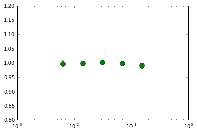
## plot ##

semilogx(fqd, fqd*0+1.0, label='input phase lag')
ylim([0.8, 1.2])
errorbar(fqd[1:-1], phi[1:-1], yerr=phie[1:-1], fmt='o', ms=10, label='fit')
<Container object of 3 artists>
