azTcl

Description

This repository contains a collection of scripts written in tcl to be used within xspec, the X-ray spectral modeling package. It contains several useful functions that streamlines some of the xspec functionality. Examples of the functions include:

• az_scan_en_norm and az_sim_dchi2: which can be used for scanning fit residuals for spectral emission or absorption lines and assessing their significance.
• az_calc_errors: Calculate the uncertainties on the fit parameters, making sure to restart if a new fit is found, save progress, and save the final results in clean manner.
• az_rand_pars: randomize the parameters given the covariance from the best fit, or give a loaded MCMC chain.
• az_rand_plot: Plot a set of models whose parameters are randomly-selected from the best fit parameters and their covariance.
• az_save_pars: return a string ($res) that has the current parameters, so that they can be loaded again quickly by doing newpar $res.
• az_best_chain_pars: return a string ($res) of the best parameters from a loaded chain. These parameters can be applied to the model by doing: newpar $res.
• az_plot_unfold: a clean and easy function to plot the unfoled data, model and their residual and ratio to a veusz-ready file.
• az_free_params: returns a list of free parameters.

Usage Example

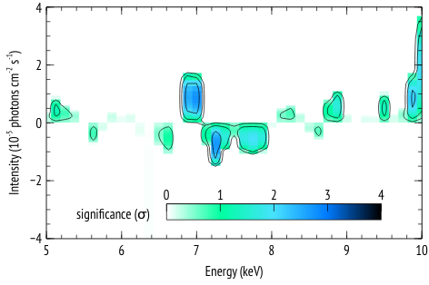
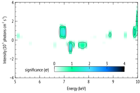
The following is an example of how the functions az_scan_en_norm and az_sim_dchi2 can be used, along with the script az_proc_scan.py to generate plots of residual significance given some best fit model to the data, similar to those in Figure 2 of this article.

The steps as presented in that paper are:

1- Start with a baseline model with its best fit chi-squared and covariance matrix (or MCMC chain) that encodes the uncertainty of best value parameters.

2- Draw N random sets of parameters using the covariance matrix (or MCMC chain if loaded).

3- For each parameter set, simulate a spectrum using the observed detector response and background files. This produces N simulated spectra that are drawn from the baseline model, taking into account its uncertainty.

4- Add a narrow Gaussian line and scan in energy and normalization and record the maximum improvement in delta-chi-squared. This gives N values of delta-chi-square that are used to construct a reference distribution to which observed delta-chi-squared values are compared. The significance of an observed delta-chi-squared is then inferred from the number of simulated fit improvement cases that have a delta-chi-squared that is as extreme as observed.

Steps

Assuming we have a file fit.xcm that loads both the data and the model, then, in xspec:

XSPEC12>source azTcl/az.tcl
XSPEC12>az_scan_en_norm fit.xcm 5 {10 5 10 40} {log 13 1e-6 1e-4 30} 1 0
XSPEC12>az_sim_dchi2 100 fit.xcm 5

Where, the first line loads the script.

The next line scans the residuals by stepping though energy (parameter number 10 from 5 to 10 keV with 40 steps) and intensity (parameter number 13 from 1e-6 to 1e-4 with 30 steps). The log before 13 indicates that the steps are in log-space. The scanning is done by adding a narrow gaussian line (component 5 in the model in this case) and stepping through the its energy and intensity values and recording the improvement in fit statistic.

Then mode=1, so that we do both positive and negative intensity values, so that both emission and absorption lines are considered. In this example, the total number of intensity values is 30 x 2 = 60.

The last number is the redshift, so the energies are in the rest-frame of the source. Here, we used 0 for illustration.

This writes a file called fit.scan that has the results of the scanning in energy and intensity

One can stop at this point and use a simple f-test to assess the significant of the residual features by calling az_proc_scan.py and giving fit.scan as input. This is however is not strictly correct (see discussion in the paper and reference therein). The reference chi-squared distribution need to be extracted from Monte-Carlo simulation that searches for features in the residuals that expected from pure noise fluctuations in the baseline model.

These simulation can be run using the command az_sim_dchi2 100 fit.xcm 5, where 100 is the number of simulated spectra (typically, one needs a larger number), fit.xcm is the file that loads the data and model, and 5 is the component number where the search gaussian is to be added.

The results will be saved: fit.sim

When running az_proc_scan.py, the code will search for a .sim file in the same location as in .scan file, and process it if found (otherwise use only the .scan file produced by az_scan_en_norm).

The result of running az_proc_scan.py is a file named fit.2d.plot that can be read by veusz for plotting. An example veusz file (.vsz) is given along with this example.

The scales and units in the plot may depend on the specific case, so the plots are given in veusz format to give the user the freedom in the plot settings.