This tutorials shows a quick guide on how to use aztools to simulated light curves similar to those observed from Astronomical objects.
Import relevant libraries and change the settings to use large plots
import numpy as np
import aztools as az
import matplotlib.pyplot as plt

# change some settings in the plot to make them clear
plt.rcParams.update({
    'font.size': 16,
    'font.family': 'monospace'
})
Now we do the simulations
# input parameters
seed = 334
n = 1024
params = [3e-5, -1, -2, 1e-3]
mu = 50
dt = 1.0

# simulation
sim = az.SimLC(seed=seed)
sim.add_model('broken_powerlaw', params)
sim.simulate(n*3, dt, mu, 'rms')
tarr, rarr = sim.t[:n], sim.x[:n]
Here we are using a broken powerlaw model for the input power spectral density, which is commenly observed.
The input parameters are:
seedis the random seed for reproducing the randomness.nis the length of the time-series needed. Note that to reproduce realistic light curves, the actual simulation is done for 3 times the length (3*n), and the only the required length is selected.mu: The mean of the resulting light curvedt: the time samplingparams: are the parameters for the input power spectral density. For the case of a broken powerlaw, the parameters are: [normalization, lowerIndex, higherIndex, breakFrequency]. The unit of the normalization is given tosim.simulateand should be one of ‘rms’, ‘var’, ‘leahy’, as defined for example in Vaughan et al. 2003.
We can also simulate another light curve that is delayed relative to the first. The lag can be in either time or phase units.
lag = 50

sim.add_model('constant', lag, lag=True)
sim.apply_lag(phase=False)
sarr = sim.y[:n]
Where we used the lag in time units (apply_lag(phase=False)), and we used a constnat lag as a function of frequency.
Using lag=True when calling add_model, tells the simulation object that we constructing a lag model and not a power spectral model.
Next we add poisson noise to the light curves (on top of the stochastic noise) to simulate the detection process.
rarr = np.random.poisson(rarr)
sarr = np.random.poisson(sarr)
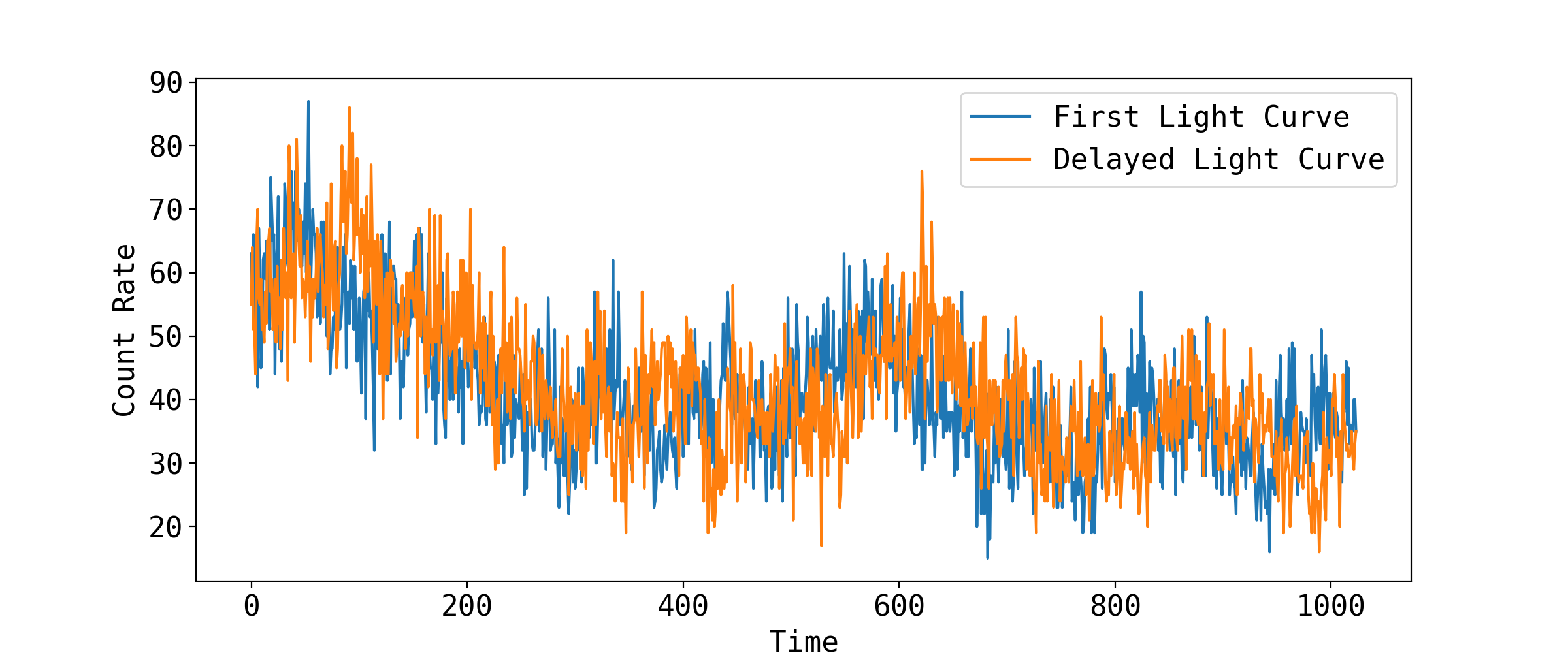
Finally, we visualize the simulated light curves
fig = plt.figure(figsize=(12,5))
plt.plot(tarr, rarr, label='First Light Curve')
plt.plot(tarr, sarr, label='Delayed Light Curve')
plt.xlabel('Time')
plt.ylabel('Count Rate')